Quantum Entanglement Primer
Objective
SAS is advancing a quantum computing initiative to bring quantum capabilities to SAS Viya. The goal is to make quantum computing more intuitive, efficient, and cost-effective, reducing the barriers to adoption and accelerating the path from experimentation to business value. This document provides a high-level introduction to the quantum physical property called entanglement that is used in quantum computing.
What Is Quantum Entanglement?
Entanglement is not faster-than-light messaging. It is a property of a joint quantum state whose correlations cannot be reproduced by a local classical model.
Quantum entanglement occurs when the joint state of two or more quantum systems cannot be written as separate states for the individual systems. The systems must be described together. Measurements on them can display correlations that cannot be reproduced by a local classical model.
Entanglement does not mean that every property of one system can be inferred from every measurement on another. The correlation depends on the entangled state and on the observables being measured. For the Bell state below, measuring both qubits in the computational basis always produces matching outcomes:
Each individual result is random. In repeated ideal measurements, half of the outcomes are \(00\) and half are \(11\). The useful structure lies in the joint distribution: the two outcomes match. If the measurement basis changes, the correlation must be analyzed in that basis.
The defining mathematical test
A pure bipartite state is entangled when it cannot be factored as \(|\Psi_{AB}\rangle=|\psi_A\rangle\otimes|\phi_B\rangle\). The complete joint state is well defined even when neither subsystem has its own pure state.
Information in correlations
A useful analogy is a quantum book whose information is stored primarily in relationships among pages rather than on any page by itself. Reading one page reveals little about the whole. The structure becomes visible only when multiple pages are examined together. Likewise, an entangled state can contain information in correlations that is absent from either subsystem alone.
Correlation is not communication
Entanglement cannot by itself transmit a controllable message faster than light. Alice cannot choose the random result recorded at one detector, and the other detector's local results are also random. The correlation appears only after the records are compared through an ordinary classical channel.
Why Entanglement Matters in Quantum Information
Entanglement gives a quantum processor access to joint states and correlations that cannot be represented as independent qubit states. Combined with superposition, relative phase, interference, and controlled operations, it can be an important resource in quantum algorithms and protocols.
- Quantum teleportation uses shared entanglement and classical communication to transfer an unknown quantum state.
- Superdense coding uses a shared Bell pair so that operations on one qubit can encode two classical bits for later joint decoding.
- Quantum networking uses entanglement as a resource for distributed quantum tasks.
- Quantum error-correcting codes encode logical information across correlated physical qubits.
- Many quantum algorithms generate entanglement, but entanglement alone does not guarantee computational advantage.
A useful explanation of quantum computation should avoid saying that the processor tries every answer in parallel and simply reads out the correct one. Measurement returns limited classical information. The algorithm must shape amplitudes and phases so that interference increases the probability of useful outcomes and suppresses others.
EPR: Is Quantum Mechanics Complete?
In 1935, Albert Einstein, Boris Podolsky, and Nathan Rosen proposed a thought experiment intended to show that quantum mechanics might be incomplete. Their argument considered two systems prepared with correlated position and momentum and then separated.
Depending on which observable is measured on system A, the corresponding observable for system B can be predicted. EPR assumed locality: a measurement choice made at A should not instantaneously disturb a distant system B. They also proposed a criterion of reality: if a physical quantity can be predicted with certainty without disturbing the system, that quantity corresponds to an element of physical reality.
Under those assumptions, EPR argued that both position and momentum should correspond to elements of reality for system B, even though quantum mechanics does not assign simultaneous definite values to both. Their conclusion was not that an experiment had violated the uncertainty principle. Their conclusion was that the quantum-mechanical description might omit additional variables needed for a complete account.
Important distinction
One cannot combine outcomes from incompatible experimental arrangements and claim that both observables were measured precisely on the same particle in the same run. The EPR argument concerns completeness, locality, and counterfactual predictions, not a direct experimental violation of the uncertainty principle.
Bell's Theorem and Experimental Tests
In 1964, John Bell showed that local hidden-variable models place limits on correlations observed when two separated experimenters choose among different measurement settings. Quantum mechanics predicts correlations that can exceed those limits for suitable entangled states and measurement choices.
The experiment in one page
- A source prepares an entangled pair and sends one system to Alice and the other to Bob.
- Alice and Bob independently choose one of two measurement settings.
- Each measurement produces one of two outcomes, represented as \(+1\) or \(-1\).
- After many trials, Alice and Bob compare their records and calculate correlations for each pair of settings.
- A local hidden-variable model must satisfy a Bell inequality. Quantum mechanics predicts a violation for selected settings.
A standard CHSH form
A widely used Bell inequality is the Clauser-Horne-Shimony-Holt, or CHSH, inequality. Let \(E(a,b)\) denote the correlation between Alice's outcome using setting \(a\) and Bob's outcome using setting \(b\). Define
Local hidden-variable models obey
Quantum mechanics allows values as large as
Repeated Bell tests have observed violations consistent with quantum predictions. The result rules out local hidden-variable explanations under the assumptions used to derive and test the inequality. It does not establish that controllable information travels faster than light, and it does not rule out every possible interpretation or every nonlocal hidden-variable theory.
Entanglement in Quantum Computing
Assumptions
Everything presented is industry standard and vendor agnostic. The illustrations below were created using the IBM Quantum Composer. This choice was made purely for convenience.
Bell States
The Bell states are four maximally entangled two-qubit states. They form an orthonormal basis for the two-qubit state space:
| State | Nonzero basis states | Computational-basis relation | Relative phase |
|---|---|---|---|
| \(\Phi^+\) | 00 and 11 | Same outcomes | Equal |
| \(\Phi^-\) | 00 and 11 | Same outcomes | Opposite |
| \(\Psi^+\) | 01 and 10 | Opposite outcomes | Equal |
| \(\Psi^-\) | 01 and 10 | Opposite outcomes | Opposite |
The plus and minus signs describe relative phase, not positive and negative probability. For every Bell state, the two nonzero computational-basis amplitudes have magnitude \(1/\sqrt{2}\), so each corresponding outcome has probability \(1/2\).
Preparing and Visualizing the Bell States
The IBM Quantum Composer screenshots show the circuit, ideal computational-basis probabilities, and Q-sphere for each Bell state. Every circuit begins in \(|00\rangle\), applies a Hadamard gate to qubit 0, and then applies a CNOT with qubit 0 as control and qubit 1 as target. Additional Pauli gates select the desired Bell state.
How to read the screenshots
The circuit appears across the top. The probability chart at lower left shows which computational-basis outcomes can be measured. The Q-sphere at lower right shows the nonzero basis-state amplitudes and their phases. Color differences in the Q-sphere distinguish relative phase, which the probability chart alone cannot reveal.
\(|\Phi^+\rangle\): matching outcomes, equal phase
The basic H-CNOT circuit prepares \(|\Phi^+\rangle\). The probability chart contains 50% at \(00\) and 50% at \(11\). The Q-sphere displays \(|00\rangle\) and \(|11\rangle\) with the same phase, corresponding to two positive amplitudes.
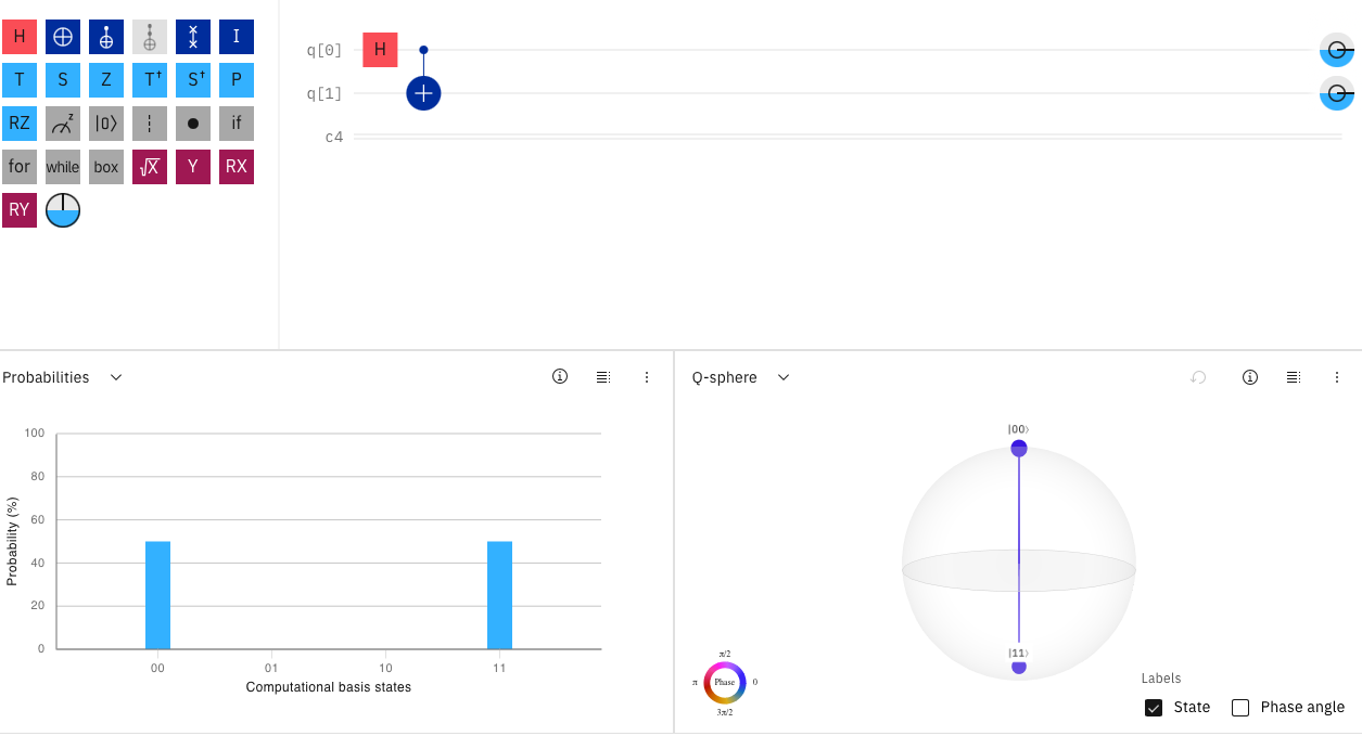
Figure 1. IBM Quantum Composer view of \(|\Phi^+\rangle\): outcomes 00 and 11 with equal probability and equal phase.
\(|\Phi^-\rangle\): matching outcomes, opposite phase
Applying \(Z\) to qubit 0 after the H-CNOT block changes the relative sign of the \(|11\rangle\) component. The probability chart remains 50% at \(00\) and 50% at \(11\) because relative phase does not change computational-basis probabilities. The Q-sphere distinguishes \(|\Phi^-\rangle\) from \(|\Phi^+\rangle\) by showing opposite phases for the two nonzero components.
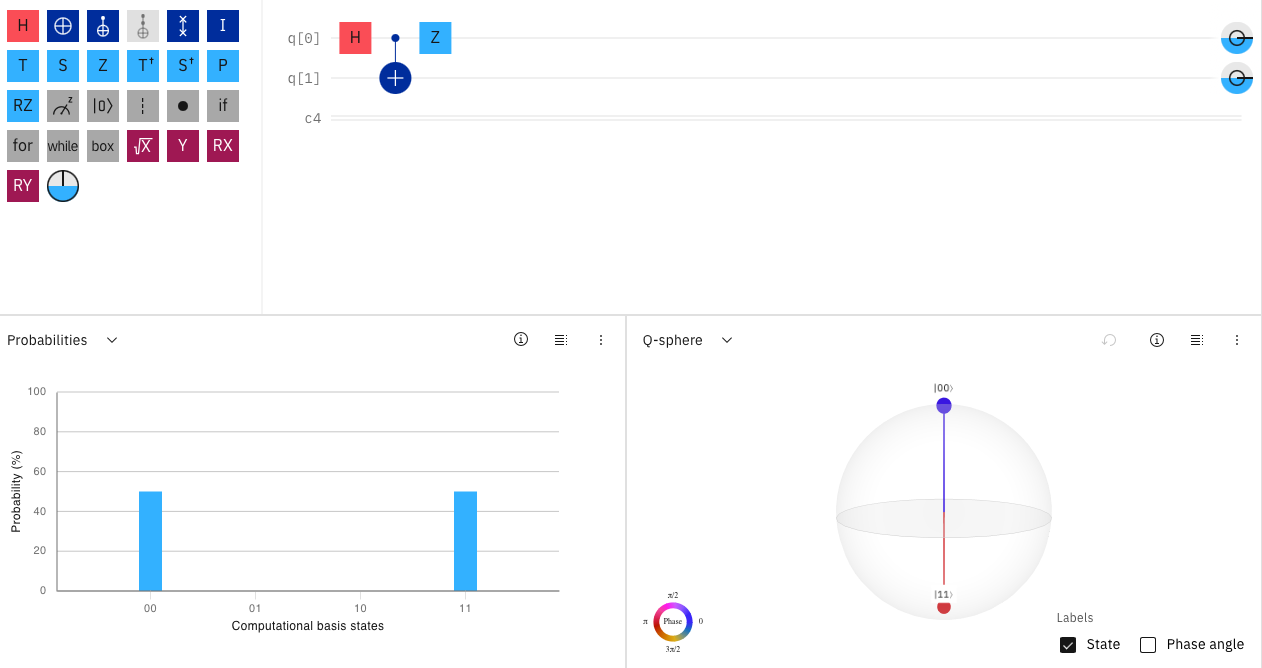
Figure 2. IBM Quantum Composer view of \(|\Phi^-\rangle\): outcomes 00 and 11 with equal probability and opposite phase.
\(|\Psi^+\rangle\): opposite outcomes, equal phase
Applying \(X\) to qubit 1 after the H-CNOT block converts same-bit correlation into opposite-bit correlation. The probability chart shifts to 50% at \(01\) and 50% at \(10\). The Q-sphere shows the \(|01\rangle\) and \(|10\rangle\) components with the same phase.
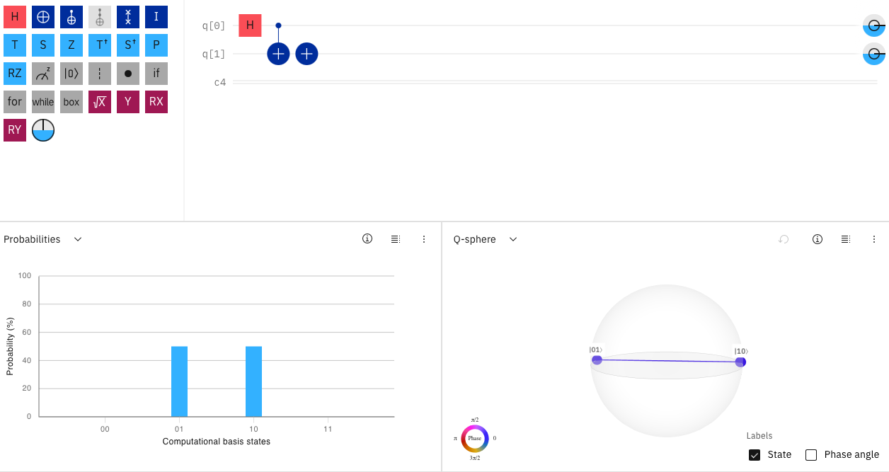
Figure 3. IBM Quantum Composer view of \(|\Psi^+\rangle\): outcomes 01 and 10 with equal probability and equal phase.
\(|\Psi^-\rangle\): opposite outcomes, opposite phase
Applying \(X\) to qubit 1 and \(Z\) to qubit 0 after the H-CNOT block prepares \(|\Psi^-\rangle\). The probability chart remains 50% at \(01\) and 50% at \(10\), while the Q-sphere shows opposite phases. As with the two \(\Phi\) states, probability alone cannot distinguish the plus and minus versions.

Figure 4. IBM Quantum Composer view of \(|\Psi^-\rangle\): outcomes 01 and 10 with equal probability and opposite phase.
What the four screenshots demonstrate
| State | Gates after H-CNOT | Nonzero outcomes | Q-sphere phase relation |
|---|---|---|---|
| \(\Phi^+\) | None | 00 and 11 | Equal |
| \(\Phi^-\) | \(Z_0\) | 00 and 11 | Opposite |
| \(\Psi^+\) | \(X_1\) | 01 and 10 | Equal |
| \(\Psi^-\) | \(X_1\) and \(Z_0\) | 01 and 10 | Opposite |
The probability charts separate the \(\Phi\) family from the \(\Psi\) family: \(\Phi\) states produce matching computational-basis outcomes, while \(\Psi\) states produce opposite outcomes. The Q-spheres separate the plus states from the minus states by revealing relative phase. This is why statevector or phase-sensitive visualization is needed in addition to measurement probabilities.
Equivalent circuit constructions
These are clean, consistent circuits, but they are not the only valid preparations. Equivalent circuits may move Pauli operations to different positions, initialize another computational-basis state before the H-CNOT block, or differ by a physically irrelevant global phase. The qubit-order convention must always be stated when comparing circuits or statevectors across software packages.
The Mathematics of \(|\Phi^+\rangle\)
Begin with two qubits in the product state
Apply a Hadamard gate to qubit 0:
Then apply the CNOT. When the control is 0, the target is unchanged. When the control is 1, the target is flipped:
The final state cannot be written as a tensor product of independent single-qubit pure states. That nonfactorability is the mathematical signature of entanglement for this pure state.
Amplitude, probability, and phase
Each nonzero Bell-state amplitude has magnitude \(1/\sqrt{2}\), and
A negative amplitude does not mean a negative probability. It indicates relative phase, which becomes observable when amplitudes later interfere. The attached probability charts therefore show identical distributions for \(\Phi^+\) and \(\Phi^-\), and likewise for \(\Psi^+\) and \(\Psi^-\), while the Q-spheres reveal the phase differences.
What local measurements see
For \(|\Phi^+\rangle\), the reduced state of either individual qubit is maximally mixed:
The complete two-qubit state is pure and fully specified, while either qubit considered alone produces an unbiased random result in the computational basis.
Interpretations versus operational descriptions
The Many-Worlds Interpretation is one interpretation of quantum mechanics, not a separate experimentally confirmed mechanism for quantum computation. Language about spawning universes or correlating universes may be used as metaphor, but it should not replace the operational account based on state preparation, unitary evolution, entanglement, interference, and measurement.
Practical framing
Entanglement is a resource, not a speedup certificate. Whether a quantum computation provides an advantage depends on the algorithm, problem structure, hardware errors, resource requirements, measurement strategy, and classical baseline.
Conclusion
Quantum entanglement is a property of a joint state that cannot be decomposed into independent states for its components. It produces correlations that can violate Bell inequalities while respecting the no-signalling requirement that prevents controllable faster-than-light communication.
The IBM Quantum Composer screenshots make the four Bell states visually distinct. The probability charts identify matching versus opposite computational-basis outcomes, while the Q-spheres expose the relative phase that distinguishes plus from minus states. A common H-CNOT block prepares \(|\Phi^+\rangle\), and simple local Pauli operations generate the remaining three states.
In quantum computing, entanglement is most powerful when used with superposition, phase, interference, and carefully designed operations. The goal is not merely to create correlated qubits, but to construct a computation in which those correlations contribute to an answer that can be extracted reliably.
Additional Resource
- Einstein, A., Podolsky, B., and Rosen, N. “Can Quantum-Mechanical Description of Physical Reality Be Considered Complete?” Physical Review 47, 1935.
- Bell, J. S. “On the Einstein Podolsky Rosen Paradox.” Physics Physique Fizika 1, 1964.
- Kaiser, D. “Bell's Inequality and Quantum Entanglement.” MIT OpenCourseWare lecture notes, 2020.
- Stanford Encyclopedia of Philosophy. “The Einstein-Podolsky-Rosen Argument in Quantum Theory.”
- Stanford Encyclopedia of Philosophy. “Quantum Entanglement and Information.”
- Caltech Science Exchange. “What Is Entanglement and Why Is It Important?”
- IBM Quantum Composer screenshots supplied by the author.