Quantum Modalities and Computational Models

A practical guide to physical qubit technologies, gate-based computing, analog simulation, and quantum annealing

Scope

This document emphasizes durable concepts rather than rapidly changing vendor rankings or raw qubit counts. System specifications should be verified directly with providers when used in presentations or purchasing decisions.

Objective

SAS is advancing a quantum computing initiative to bring quantum capabilities to SAS Viya. The goal is to make quantum computing more intuitive, efficient, and cost-effective, reducing the barriers to adoption and accelerating the path from experimentation to business value. This document provides a high-level introduction to the major quantum computing modalities and computational models.

1. Introduction

Quantum computing is not based on a single hardware architecture. Different systems encode and manipulate quantum information using atoms, ions, photons, electron or nuclear spins, superconducting circuits, or proposed topological states. These physical implementations are often called qubit modalities.

The physical modality is only one part of a quantum computer. Systems also differ in their computational model: the way a problem is represented, controlled, and executed. Major models include gate-based quantum computing, analog quantum simulation, and quantum annealing. Some hardware platforms support more than one model.

No modality or model is best for every application. Each involves trade-offs among state preparation, coherence, gate or control fidelity, connectivity, measurement, operating environment, programmability, scalability, and accessibility. Comparing platforms therefore requires more than comparing raw qubit counts.

Three terms to keep separate

Modality identifies the physical carrier of quantum information.
Computational model describes how a computation is expressed and executed.
Architecture describes how qubits, controls, couplers, measurement, and supporting systems are organized within a particular implementation.

1.1 How to read this guide

1. Section 2 compares the principal physical qubit modalities.
2. Section 3 explains the major computational models.
3. Section 4 shows how modality and model interact in practice.
4. Section 5 provides a concise framework for evaluating systems without relying on a single headline metric.

Modality, information carrier, control, and computational model

Modality	Information carrier	Typical control	Common model
Neutral atoms	Selected atomic states	Lasers and optical tweezers	Analog and gate-based
Trapped ions	Electronic or hyperfine states of ions	Lasers, RF fields, and electrode voltages	Gate-based
Semiconductor spins	Electron or hole spin states	Microwave, magnetic, and electric control	Gate-based
Diamond NV centers	Electron and nearby nuclear spins	Optical and microwave control	Gate-based and networking
Photonics	Discrete photons or optical modes	Sources, interferometers, phase control, and detectors	Sampling, measurement-based, and gate-based
Superconducting circuits	Quantized circuit energy states	Microwave and flux control	Gate-based and annealing
Topological approaches	Nonlocal encoded quantum states	Proposed topological operations	Gate-based, proposed

Principal strengths and challenges

Modality	Principal strength	Principal challenge
Neutral atoms	Reconfigurable arrays and strong Rydberg interactions	Atom loss, calibration, and high-fidelity control
Trapped ions	High-fidelity operations and strong connectivity	Gate speed and system-level scaling
Semiconductor spins	Small device size and semiconductor compatibility	Uniform fabrication and control at scale
Diamond NV centers	Long-lived spin states and optical interfaces	Scalable coupling and fabrication consistency
Photonics	Low decoherence in transmission	Optical loss and resource overhead
Superconducting circuits	Fast operation and mature control stack	Cryogenics, noise, and limited coherence
Topological approaches	Potential intrinsic protection from local noise	Experimental realization and validation

Quantum Modalities & Computation Models

2. Physical Qubit Modalities

A qubit is a controllable two-level quantum system used to encode a computational basis. The labels 0 and 1 refer to two selected quantum states, not necessarily to literal particles pointing in fixed directions. A useful modality must support reliable initialization, control, interaction, and measurement while preserving quantum information long enough to perform meaningful operations.

2.1 Neutral atoms

Neutral-atom quantum computers commonly use atoms such as rubidium or strontium. Focused laser beams called optical tweezers trap individual atoms and arrange them into programmable geometries. Quantum information is encoded in selected internal atomic states chosen for stability, controllability, and readout.

For entangling operations, atoms can be excited to high-energy Rydberg states. These states produce strong interactions between nearby atoms, allowing the behavior of one atom to depend on the state of another. The combination of reconfigurable atom placement and controllable Rydberg interactions makes the platform attractive for both analog simulation and gate-based processing.

• Strengths: Large and reconfigurable arrays, flexible interaction geometry, and support for more than one computational model.
• Challenges: Atom preparation and loss, laser stability, calibration across large arrays, and consistently high-fidelity operations.

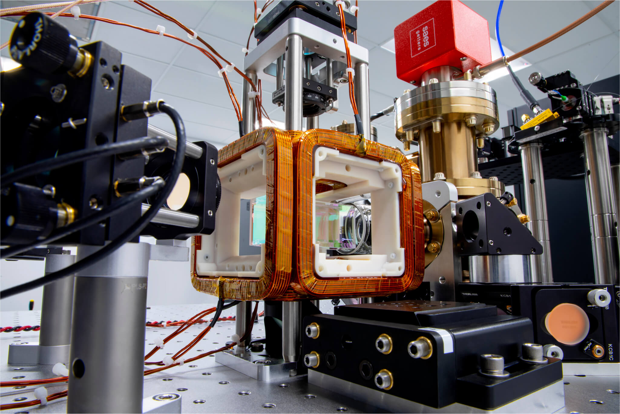
Figure 1. Neutral-atom experimental system.

2.2 Semiconductor spin qubits

Semiconductor spin qubits confine electrons or holes in small regions of semiconductor material, often called quantum dots. Two selected spin states encode the computational basis. Microwave, magnetic, and electric controls manipulate the states, while nearby gates and sensors support confinement and readout.

The approach is attractive because the devices are physically small and may benefit from established semiconductor fabrication techniques. The central challenge is producing large numbers of nearly identical devices and controlling them without introducing excessive wiring, cross-talk, or variation.

• Strengths: Compact qubits, compatibility with semiconductor engineering, and potential for dense integration.
• Challenges: Device variability, cryogenic control, coupling over distance, and calibration at scale.

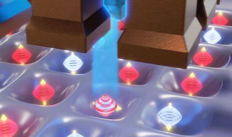
Figure 2. Conceptual control of localized semiconductor spin qubits.

2.3 Trapped ions

Trapped-ion quantum computers use charged atoms confined by electromagnetic fields. Quantum information is stored in selected electronic or hyperfine states. Lasers prepare, manipulate, entangle, and measure the ions. In segmented trap architectures, changing DC electrode voltages can transport ions between storage, gate, and measurement zones.

Because ions of the same species are naturally identical, trapped-ion systems can achieve uniform qubits and high-quality operations. Collective vibrational motion or other imgted interactions can provide effective connectivity among ions. Scaling requires careful engineering of transport, optical delivery, control electronics, and error management.

• Strengths: Uniform qubits, high-fidelity operations, long coherence, and strong effective connectivity.
• Challenges: Slower operations than some solid-state platforms, complex optical systems, and scaling control across many ions.

Figure 3. Microfabricated trapped-ion structure.

2.4 Nitrogen-vacancy centers in diamond

A nitrogen-vacancy center is a defect in diamond formed by a nitrogen atom adjacent to a missing carbon atom. The defect supports electronic spin states that can encode quantum information. Nearby nuclear spins may provide additional qubits or longer-lived quantum memory.

Optical signals support initialization and readout, while microwave fields control the electron spin. The combination of spin coherence and an optical interface makes NV centers relevant not only to computing, but also to sensing and quantum networking. The principal difficulty is creating uniform devices and coupling many centers into a scalable architecture.

• Strengths: Long-lived spin states, optical access, and potential integration of processing, memory, sensing, and networking.
• Challenges: Deterministic fabrication, photon collection, spectral consistency, and scalable interactions between distant centers.

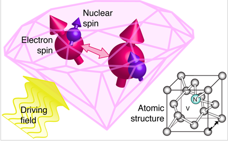
Figure 4. Electron and nuclear spins associated with a diamond defect.

2.5 Photonics

Photonic quantum computers use photons or optical modes to carry quantum information. Depending on the architecture, information may be encoded in optical path, polarization, time bins, frequency bins, photon number, or continuous-variable optical quadratures. This diversity is important: no single source-interferometer-detector description covers every photonic system.

In a continuous-variable architecture, squeezed-light sources prepare nonclassical optical states, programmable interferometers transform the modes, and photon-number-resolving or homodyne detectors produce measurement outcomes. Other photonic approaches rely on single-photon sources, fusion operations, or measurement-based resource states.

• Strengths: Transmission at or near room temperature, natural compatibility with optical networking, and low decoherence during propagation.
• Challenges: Photon loss, source and detector efficiency, probabilistic operations in some architectures, and large resource overhead for fault tolerance.

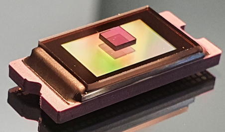
Figure 5. Example photonic pipeline with sources, interferometer, and detection.

2.6 Superconducting circuits

Superconducting quantum processors use nonlinear electrical circuits operated at millikelvin temperatures. A Josephson junction provides the nonlinearity required to create discrete, addressable energy levels. Two selected levels form the computational basis, and microwave or flux-control signals implement operations and readout.

Different superconducting qubit designs encode information in different circuit variables. For example, transmon qubits primarily use quantized energy levels of a nonlinear oscillator, while flux-qubit designs emphasize circulating-current states. A general description should therefore avoid treating current direction as the universal meaning of 0 and 1.

Superconducting technology supports both gate-based processors and quantum annealers, but those systems should not be compared solely by physical-qubit count. Their connectivity, control model, error behavior, and supported workloads are fundamentally different.

• Strengths: Rapid operations, lithographic fabrication, established microwave control, and a broad software ecosystem.
• Challenges: Dilution refrigeration, environmental noise, fabrication variability, limited coherence, and wiring complexity.

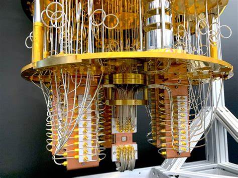
Figure 6. Packaged superconducting quantum processor.

2.7 Topological approaches

Topological quantum computing seeks to encode information nonlocally in collective quantum states. In the most familiar proposal, logical operations would be performed by exchanging, or braiding, non-Abelian excitations. Their trajectories through two spatial dimensions over time form braids in 2+1-dimensional spacetime.

Because the information would be represented in global properties of the system, local disturbances may have less effect on the encoded state. This is the central attraction of the approach. However, creating, controlling, and validating a scalable topological processor remains a major research challenge, so proposed advantages should be presented as goals rather than established system-level capabilities.

• Potential strength: Intrinsic protection against some local errors, which could reduce error-correction overhead.
• Primary challenge: Experimentally demonstrating and scaling the required physical states and operations.

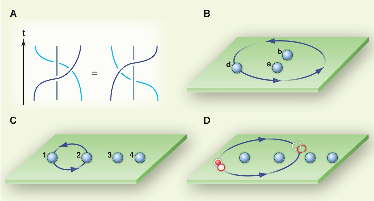
Figure 7. Conceptual worldlines that form a braid.

3. Computational Models

A computational model defines how a user expresses a problem and how the physical system evolves to produce a result. The terms gate-based, analog, and annealing describe models of computation, not physical qubit modalities. The same modality may support multiple models, and similar models may be implemented with different modalities.

3.1 Gate-based quantum computing

Gate-based quantum computing represents a program as a circuit composed of quantum operations applied to qubits. Single-qubit gates change individual states, multi-qubit gates create correlations and entanglement, and measurement converts selected quantum information into classical outcomes. Compilers translate the logical circuit into operations supported by the target hardware.

The circuit is a digital abstraction, but the physical hardware implements each gate using continuously varying control signals. It is therefore more accurate to say that a discrete gate model is realized by analog physical controls than to say that every digital program is converted into an analog-computing problem.

!!! note "Circuit terminology
Width is the number of qubits used by a circuit. Depth is the number of sequential operation layers after gates that can execute in parallel are grouped together. Gate count is the total number of operations. These quantities are related but are not interchangeable.

As circuits become deeper, accumulated control errors, measurement errors, cross-talk, and decoherence can degrade the output. The usable depth depends on the hardware, circuit structure, compilation, and error-management techniques. Error mitigation can improve estimates in some cases, while fault-tolerant error correction is intended to support reliable computations at much greater scale.

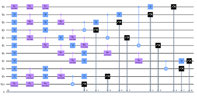
Figure 8. Quantum circuit with single-qubit and entangling operations.

3.2 Analog quantum computing and simulation

Analog quantum computing programs the continuous evolution of a quantum system so that its Hamiltonian represents or approximates a physical system or computational problem. Instead of decomposing the entire computation into a standard sequence of discrete gates, the user controls interactions, fields, detunings, or other physical parameters over time.

Analog systems can use hardware efficiently when a problem aligns with the platform's native interactions. This can be especially useful for quantum simulation and certain optimization formulations. The trade-off is specialization: the user may need more knowledge of the device physics, available controls, and mathematical model, and the same system may not implement arbitrary algorithms in the way a universal gate-based processor can.

• Good fit: Simulation of quantum dynamics, many-body physics, and selected optimization problems.
• Key consideration: Performance depends strongly on how naturally the target Hamiltonian maps onto the available hardware.

3.3 Quantum annealing

Quantum annealing is a specialized analog approach used primarily for optimization and sampling problems that can be expressed as an Ising model or a quadratic unconstrained binary optimization model. The process begins with a driver Hamiltonian whose low-energy state is easy to prepare and gradually replaces it with a problem Hamiltonian whose low-energy states encode high-quality solutions.

\[ H(s)=A(s)H_D+B(s)H_P, \qquad 0 \le s \le 1 \]

Here, \(H_D\) is the driver Hamiltonian and \(H_P\) is the problem Hamiltonian. During a standard forward anneal, \(A(s)\) decreases while \(B(s)\) increases. If the evolution is sufficiently controlled, the system tends to remain near low-energy states of the evolving Hamiltonian. At the end of the anneal, measurement returns samples and their associated energies.

The returned samples are candidate solutions, not automatic guarantees of global optimality. Results can be affected by finite temperature, noise, control error, anneal schedule, embedding, chain breaks, and the structure of the energy landscape. Practical applications often combine the quantum processing unit with classical preprocessing, decomposition, postprocessing, or hybrid solvers.

• Strength: Direct mapping of binary optimization models onto a specialized physical process.
• Limitation: The model addresses a narrower problem class than general gate-based computing.
• Evaluation principle: Compare complete workflows, including modeling, embedding, repeated sampling, classical processing, solution quality, and wall-clock cost.

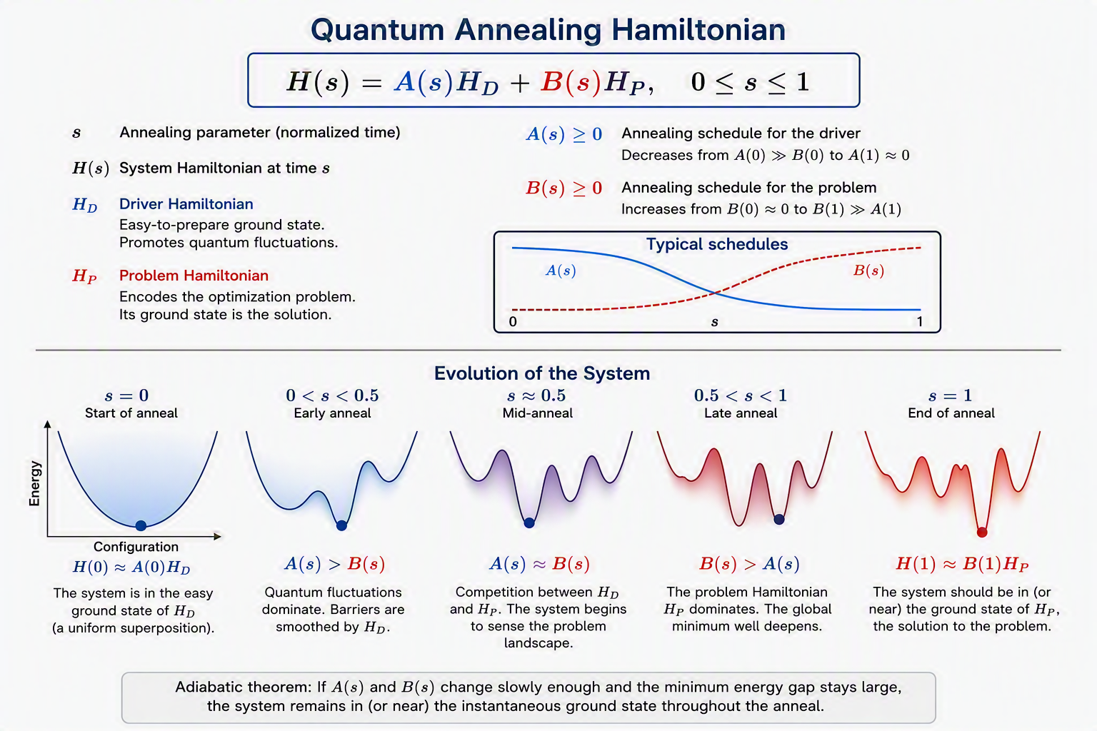
Figure 9. Example of quantum annealing process

3.4 Hybrid analog-digital approaches

The boundary between computational models is not always sharp. A system may use analog blocks inside a gate-based workflow, digital controls around analog evolution, or classical optimization around repeated quantum executions. Hybrid designs can exploit hardware-native operations while retaining higher-level programmability.

For users, the practical question is not whether a platform is purely digital or purely analog. The more useful questions are what problem representations it supports, how much control it exposes, which operations are native, and what classical processing is required before and after quantum execution.

4. Relating Modality to Computational Model

Modality and model should be evaluated together. A physically attractive qubit is not automatically the best platform for a particular algorithm, and a compelling computational model is not automatically efficient on every implementation.

Platform family	Gate-based	Analog simulation	Annealing
Neutral atoms	Supported by several architectures	Strong fit for programmable interactions	Possible formulations, platform dependent
Trapped ions	Primary model	Possible, especially simulation	Not the principal commercial model
Semiconductor spins	Primary research direction	Possible in specialized designs	Not the principal model
Diamond NV centers	Research direction	Possible for specialized simulation	Not the principal model
Photonics	Several approaches	Continuous-variable and sampling approaches	Not the principal model
Superconducting circuits	Widely used	Possible with native interactions	Commercially established
Topological approaches	Proposed logical-gate model	Not the principal framing	Not the principal framing

Important

This table describes broad associations, not rigid boundaries. Implementations evolve, and individual providers may support capabilities beyond the dominant model associated with a modality.

5. A Better Way to Compare Quantum Systems

Raw qubit count is easy to communicate but rarely sufficient for technical evaluation. A useful comparison should begin with the workload and then assess the complete system against the requirements of that workload.

5.1 Start with the problem

• Is the objective simulation, optimization, sampling, machine learning, cryptanalysis, or another workload?
• Can the problem be expressed naturally in the platform's supported representation?
• What solution quality, confidence, latency, throughput, and cost are required?
• What classical preprocessing and postprocessing are part of the workflow?

5.2 Evaluate the hardware in context

• Qubit or mode quality: Coherence, gate or control fidelity, calibration stability, and measurement quality.
• Connectivity: Which pairs can interact directly, and what routing or embedding overhead is required?
• Effective problem size: How many logical variables or useful degrees of freedom remain after encoding, routing, error management, or embedding?
• Control and programmability: Which operations are native, and which must be synthesized or approximated?
• Availability and reproducibility: Access model, queueing, calibration variability, tooling, and repeatability.

5.3 Compare complete workflows

The relevant benchmark is the full path from problem definition to validated answer. Quantum execution time alone can omit model construction, compilation, embedding, data movement, repeated sampling, error mitigation, and classical postprocessing. Comparisons should use clearly defined baselines and report both solution quality and total resource cost.

6. Conclusion

Quantum computing comprises multiple physical modalities and computational models. Neutral atoms, trapped ions, semiconductor spins, diamond defects, photons, superconducting circuits, and proposed topological states offer different paths to creating and controlling qubits. Gate-based computing, analog simulation, and quantum annealing provide different ways to express and execute computations.

The most productive question is not which modality has the largest number of qubits. It is which combination of modality, architecture, computational model, software, and classical support best matches the problem being solved. That framing produces comparisons that are more technically meaningful and more durable than vendor rankings or rapidly changing device specifications.